第13章 回帰分析における推定と検定

13.1 単回帰分析

carsデータを使う．散布図

plot(cars$speed,cars$dist)

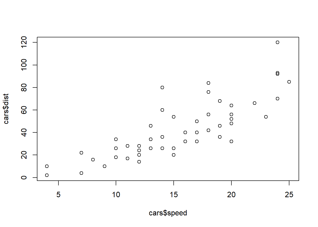
speedを独立変数，distを従属変数とする回帰分析を実行する．

lm_cars<-lm(dist ~ speed, data=cars)
slm_cars<-summary(lm_cars)
slm_cars

## 
## Call:
## lm(formula = dist ~ speed, data = cars)
## 
## Residuals:
##     Min      1Q  Median      3Q     Max 
## -29.069  -9.525  -2.272   9.215  43.201 
## 
## Coefficients:
##             Estimate Std. Error t value Pr(>|t|)    
## (Intercept) -17.5791     6.7584  -2.601   0.0123 *  
## speed         3.9324     0.4155   9.464 1.49e-12 ***
## ---
## Signif. codes:  0 '***' 0.001 '**' 0.01 '*' 0.05 '.' 0.1 ' ' 1
## 
## Residual standard error: 15.38 on 48 degrees of freedom
## Multiple R-squared:  0.6511,	Adjusted R-squared:  0.6438 
## F-statistic: 89.57 on 1 and 48 DF,  p-value: 1.49e-12

\(t\)値を係数と標準誤差から計算してみる．

t<-slm_cars$coefficients["speed","Estimate"]/slm_cars$coefficients["speed","Std. Error"]
t

## [1] 9.46399

2*(1-pt(abs(t),nrow(cars)-1-1))

## [1] 1.489919e-12

回帰直線をプロット．

plot(cars$speed,cars$dist,col="lightgrey")
abline(coef=coef(lm_cars),col="red",lwd=2)

最適化optim関数を使って，自力で最小二乗法を実行する．

sumsq<-function(coef) sum((cars$dist-coef[[1]]-coef[[2]]*cars$speed)^2)
optim(c(0,0),sumsq)

## $par
## [1] -17.571729   3.931832
## 
## $value
## [1] 11353.52
## 
## $counts
## function gradient 
##       91       NA 
## 
## $convergence
## [1] 0
## 
## $message
## NULL

分散共分散から係数を求める．

cov_cars<-cov(cars)
mean_speed<-mean(cars$speed)
mean_dist<-mean(cars$dist)

c(mean_dist-cov_cars[1,2]*mean_speed/cov_cars[1,1],
  cov_cars[1,2]/cov_cars[1,1])

## [1] -17.579095   3.932409

13.2 重回帰分析

mtcarsデータを使う

head(mtcars)

##                    mpg cyl disp  hp drat    wt  qsec vs am gear carb
## Mazda RX4         21.0   6  160 110 3.90 2.620 16.46  0  1    4    4
## Mazda RX4 Wag     21.0   6  160 110 3.90 2.875 17.02  0  1    4    4
## Datsun 710        22.8   4  108  93 3.85 2.320 18.61  1  1    4    1
## Hornet 4 Drive    21.4   6  258 110 3.08 3.215 19.44  1  0    3    1
## Hornet Sportabout 18.7   8  360 175 3.15 3.440 17.02  0  0    3    2
## Valiant           18.1   6  225 105 2.76 3.460 20.22  1  0    3    1

hpとwtよりmpgを説明する．

lm_mtcars <- lm(mpg ~ hp + wt, data=mtcars)
slm_mtcars<-summary(lm_mtcars)
slm_mtcars

## 
## Call:
## lm(formula = mpg ~ hp + wt, data = mtcars)
## 
## Residuals:
##    Min     1Q Median     3Q    Max 
## -3.941 -1.600 -0.182  1.050  5.854 
## 
## Coefficients:
##             Estimate Std. Error t value Pr(>|t|)    
## (Intercept) 37.22727    1.59879  23.285  < 2e-16 ***
## hp          -0.03177    0.00903  -3.519  0.00145 ** 
## wt          -3.87783    0.63273  -6.129 1.12e-06 ***
## ---
## Signif. codes:  0 '***' 0.001 '**' 0.01 '*' 0.05 '.' 0.1 ' ' 1
## 
## Residual standard error: 2.593 on 29 degrees of freedom
## Multiple R-squared:  0.8268,	Adjusted R-squared:  0.8148 
## F-statistic: 69.21 on 2 and 29 DF,  p-value: 9.109e-12

\(t\)値を確認する．

t_hp<-slm_mtcars$coefficients["hp","Estimate"]/slm_mtcars$coefficients["hp","Std. Error"]
t_hp

## [1] -3.518712

2*(1-pt(abs(t_hp),nrow(mtcars)-2-1))

## [1] 0.001451229

t_wt<-slm_mtcars$coefficients["wt","Estimate"]/slm_mtcars$coefficients["wt","Std. Error"]
t_wt

## [1] -6.128695

2*(1-pt(abs(t_wt),nrow(mtcars)-2-1))

## [1] 1.119647e-06

\(F\)値も確認する．

F<-slm_mtcars$r.squared/(1-slm_mtcars$r.squared)*(nrow(mtcars)-2-1)/2
F

## [1] 69.21121

1-pf(F,2,nrow(mtcars)-2-1)

## [1] 9.109047e-12

以下参考．回帰係数を自力で求める． c.f 永田靖・棟近雅彦，2001，『多変量解析法入門』サイエンス社．

X<-cbind(rep(1,nrow(mtcars)),mtcars$hp,mtcars$wt)

XX<-t(X)%*%X
Xy<-t(X)%*% mtcars$mpg
solve(XX) %*% Xy

##             [,1]
## [1,] 37.22727012
## [2,] -0.03177295
## [3,] -3.87783074