第9章 統計的推定(2): 区間推定

set.seed(8931)

9.1 正規分布からのランダムサンプリング

\(N(165,10)\)から\(n=10\)のランダムサンプリングを行って95%信頼区間を推定する．

ex<-rnorm(10,165,10)
m<-mean(ex)
ci<-1.96*sd(ex)/sqrt(10)
c(m-ci,m,m+ci)

## [1] 161.4834 168.4489 175.4144

9.2 ランダムサンプリングの繰り返し

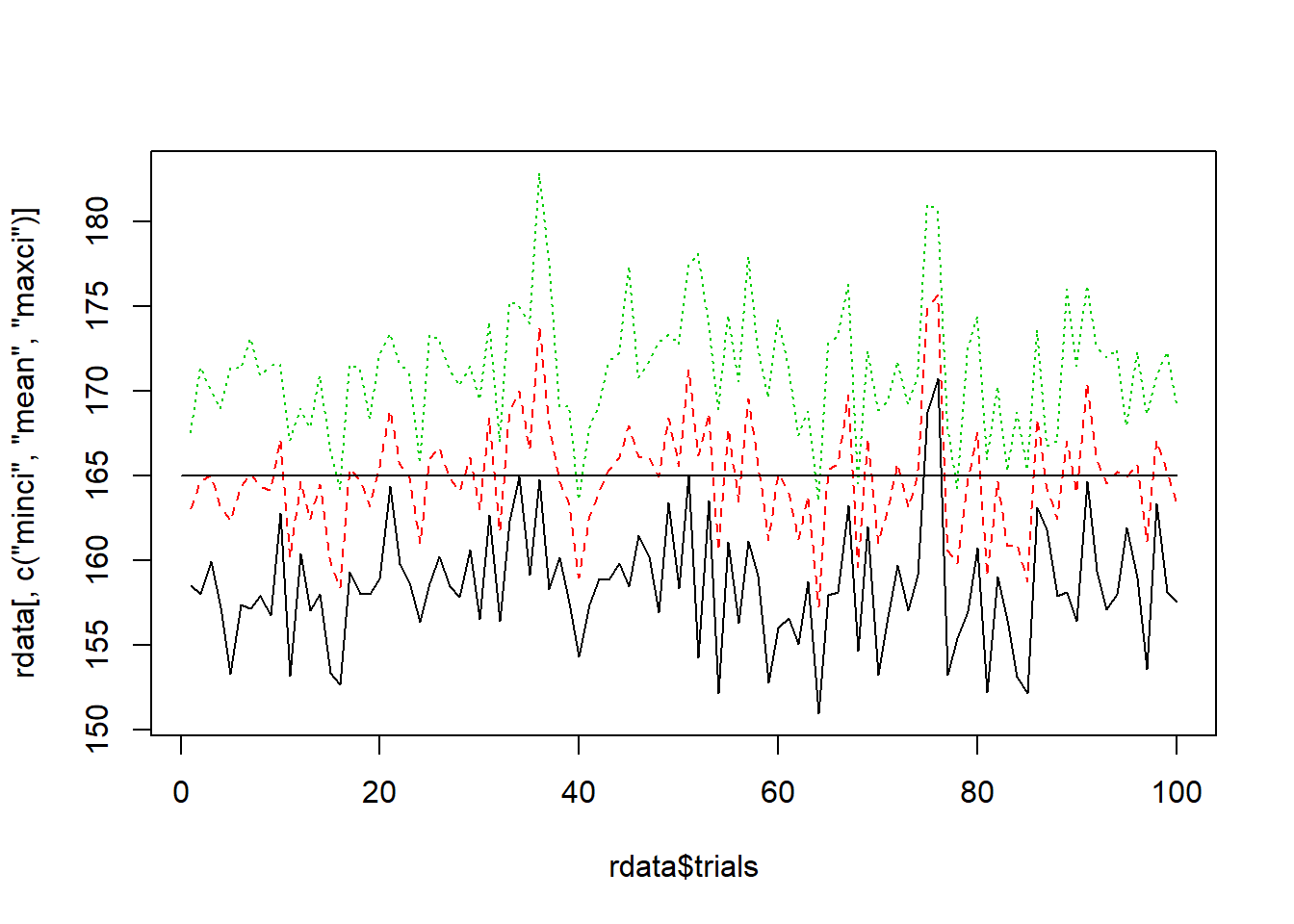
95%信頼区間の推定を100回繰り返す．

rdata<-replicate(100,{
  ex<-rnorm(10,165,10)
  m<-mean(ex)
  ci<-1.96*sd(ex)/sqrt(10)
  c(m-ci,m,m+ci)
})
rdata<-data.frame(1:100,t(rdata))
colnames(rdata)<-c("trials","minci","mean","maxci")
head(rdata)

##   trials    minci     mean    maxci
## 1      1 158.5386 163.0471 167.5556
## 2      2 158.0395 164.7257 171.4119
## 3      3 159.9578 164.9774 169.9970
## 4      4 157.2232 163.1067 168.9902
## 5      5 153.2887 162.3171 171.3455
## 6      6 157.3803 164.3814 171.3826

作図してみてみよう．

matplot(rdata$trials, rdata[,c("minci","mean","maxci")], type="l")
segments(0,165,100,165)

正答率を算出する．

sum(rdata$minci<165 & rdata$maxci > 165)/100

## [1] 0.92

ggplot2でかっこよく作図する．

library(ggplot2)
ggplot(data = rdata, aes(x = mean ,y = trials)) + 
  geom_point() + 
  geom_errorbarh(aes(xmin=minci, xmax=maxci)) +
  geom_vline(xintercept = 165, color="red")

関数化（要gglpot2）．m: 正規分布の平均，s: 正規分布の標準偏差，n: サンプルサイズ，r: 繰り返し回数

CItest<-function(m,s,n,r) {
  rdata<-replicate(r,{
    ex<-rnorm(n,m,s)
    m<-mean(ex)
    ci<-1.96*sd(ex)/sqrt(n)
    c(m-ci,m,m+ci)
  })
  rdata<-data.frame(1:r,t(rdata))
  colnames(rdata)<-c("trials","minci","mean","maxci")
  sr<-sum(rdata$minci<m & rdata$maxci > m)/r
  cat(paste("正答率: ",sr))
  ggplot2::ggplot(data = rdata, aes(x = mean ,y = trials)) + 
    geom_point() + 
    geom_errorbarh(aes(xmin=minci, xmax=maxci)) +
    geom_vline(xintercept = m, color="red")
}
CItest(160,20,10,500)

## 正答率:  0.92